
The observation
Every retail trader has had this moment. You are staring at the charts, and you notice a rhythm. The price shoots up, pulls back slightly, and then continues its run. You see it happen over and over again. You think to yourself: "If I just buy the pullback, I'll win 8 out of 10 times."
It feels like finding the Holy Grail. So, you write an Expert Advisor (EA), run a backtest, and… the equity curve is a straight line down. You are left baffled. How can a pattern that works visually fail so miserably in execution?
Recently, we took this exact visual observation — specifically on GBPUSD, a major forex pair — and subjected it to rigorous quantitative analysis. We downloaded historical intraday data, wrote Python scripts to measure the precise probabilities, and tested multiple automated strategies.
What we found is a masterclass in the difference between a statistical probability and a tradeable edge.
Here is the breakdown, complete with the Python code, so you can reproduce these tests and see the data for yourself. We used Google Colab for our Jupyter test lab.
Step 0: The data (GBPUSD)
To reproduce these tests, we will use the dukascopy_python
library, which provides free, high-quality historical forex data.
We used Google Colab for our Jupyter playground.
The Python code:
# Install required libraries (Run this first in Colab/Jupyter)
!pip install dukascopy-python pandas numpy matplotlib seaborn
import pandas as pd
import numpy as np
import matplotlib.pyplot as plt
import seaborn as sns
from datetime import datetime
import dukascopy_python
from dukascopy_python.instruments import INSTRUMENT_FX_MAJORS_GBP_USD
# Download 1 year of 5-minute (M5) data
START = datetime(2025, 1, 1)
END   = datetime(2025, 12, 31)
df = dukascopy_python.fetch(
    instrument = INSTRUMENT_FX_MAJORS_GBP_USD,
    interval   = dukascopy_python.INTERVAL_MIN_5,
    offer_side = dukascopy_python.OFFER_SIDE_BID,
    start      = START,
    end        = END,
)
df = df[['open', 'high', 'low', 'close', 'volume']].copy()
df.index.name = 'timestamp'
df = df.sort_index()
print(f"Downloaded {len(df):,} bars.")
Test 1: The "Goldilocks" zone (continuation probability)
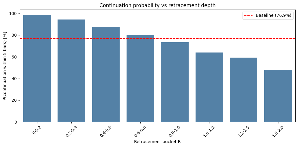
This chart is the empirical proof of the retail trader's visual observation. It measures the likelihood that the price will continue in its original direction within the next 5 bars, based on how deeply it has pulled back (measured as a fraction of the prior bar's total range, or "R").
The results
- Baseline: if you do nothing and just wait 5 bars, the price touches the prior high/low 77.3% of the time.
- 0.4 to 0.6 bucket: when the price retraces between 40% and 60%, the continuation probability spikes to 87.4%.
- > 1.0 bucket: when the price breaks the prior extreme, continuation drops to 63%, and eventually to 47% at the 1.5–2.0 mark.
The Python code:
# Calculate the Prior Bar's Direction and Range
df['prior_dir'] = np.sign(df['close'].shift(1) - df['open'].shift(1))
df['prior_high'] = df['high'].shift(1)
df['prior_low'] = df['low'].shift(1)
df['prior_range'] = df['prior_high'] - df['prior_low']
# Calculate R (Retracement depth)
R_up = (df['prior_high'] - df['low']) / df['prior_range']
R_down = (df['high'] - df['prior_low']) / df['prior_range']
df['R'] = np.where(df['prior_dir'] == 1, R_up, R_down)
# Look ahead 5 bars to see if price hits the prior extreme
N = 5
df['future_high'] = df['high'].rolling(N).max().shift(-N)
df['future_low'] = df['low'].rolling(N).min().shift(-N)
# Continuation logic
df['continuation'] = np.where(
    df['prior_dir'] == 1,
    df['future_high'] > df['prior_high'], # Bullish prior bar -> new high
    df['future_low'] < df['prior_low']    # Bearish prior bar -> new low
)
# Bucket the R values and calculate probability
df_clean = df.dropna().copy()
df_clean['R'] = df_clean['R'].clip(lower=0, upper=2.0)
bins = [0, 0.2, 0.4, 0.6, 0.8, 1.0, 1.2, 1.5, 2.0]
labels = ['0-0.2','0.2-0.4','0.4-0.6','0.6-0.8','0.8-1.0','1.0-1.2','1.2-1.5','1.5-2.0']
df_clean['R_bucket'] = pd.cut(df_clean['R'], bins=bins, labels=labels)
cont_prob = df_clean.groupby('R_bucket', observed=True)['continuation'].mean() * 100
baseline = df_clean['continuation'].mean() * 100
# Plotting Chart 1
plt.figure(figsize=(10, 5))
ax = sns.barplot(x=cont_prob.index, y=cont_prob.values, color='steelblue')
plt.axhline(baseline, color='red', linestyle='--', label=f'Baseline ({baseline:.1f}%)')
plt.title('Continuation probability vs retracement depth')
plt.xlabel('Retracement bucket R')
plt.ylabel('P(continuation within 5 bars) [%]')
plt.xticks(rotation=45)
plt.legend()
plt.tight_layout()
plt.show()
Test 2: The universal truth (session & volatility)
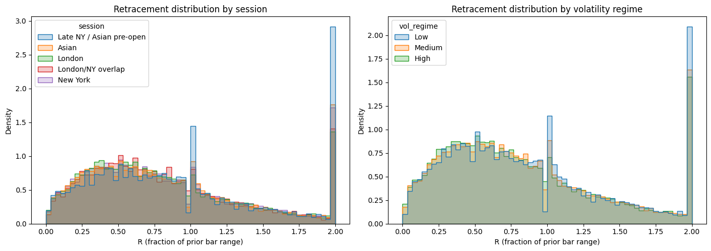
Before building a strategy, you need to know if this edge is a fluke. Does it only happen during the London session? Does it disappear during high volatility? This chart proves it doesn't. The median retracement is around 70% across every single session and every volatility regime.
The Python code:
# Define sessions (UTC)
def get_session(h):
    if 0 <= h < 8: return 'Asian'
    elif 8 <= h < 13: return 'London'
    elif 13 <= h < 16: return 'London/NY overlap'
    elif 16 <= h < 21: return 'New York'
    else: return 'Late NY / Asian pre-open'
df_clean['session'] = df_clean.index.hour.map(get_session)
# Define Volatility (ATR)
df_clean['tr'] = np.maximum(df_clean['high'] - df_clean['low'],
             np.maximum(abs(df_clean['high'] - df_clean['close'].shift(1)),
                        abs(df_clean['low'] - df_clean['close'].shift(1))))
df_clean['atr14'] = df_clean['tr'].rolling(14).mean()
df_clean['vol_regime'] = pd.qcut(df_clean['atr14'], q=3, labels=['Low', 'Medium', 'High'])
# Plotting Chart 2
fig, axes = plt.subplots(1, 2, figsize=(14, 5))
# Session histogram
sns.histplot(data=df_clean, x='R', hue='session', bins=60, element='step', stat='density', common_norm=False, ax=axes[0])
axes[0].set_title('Retracement distribution by session')
axes[0].set_xlabel('R (fraction of prior bar range)')
# Volatility histogram
sns.histplot(data=df_clean, x='R', hue='vol_regime', bins=60, element='step', stat='density', common_norm=False, ax=axes[1])
axes[1].set_title('Retracement distribution by volatility regime')
axes[1].set_xlabel('R (fraction of prior bar range)')
plt.tight_layout()
plt.show()
Test 3: The whipsaw trap (the path of pain)
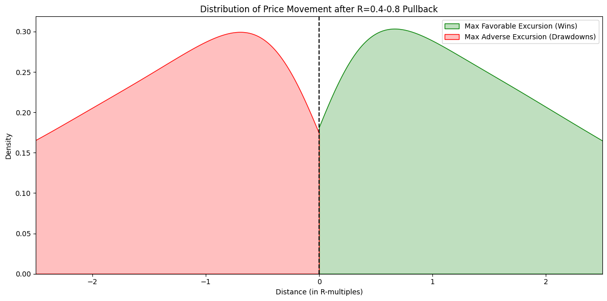
If you have an 87% edge, why do automated EAs lose money? This chart measures the Maximum Adverse Excursion (MAE) — how far the trade goes against you — and the Maximum Favourable Excursion (MFE) — how far it goes in your favour.
The data proves that the average move against you is -2.27 R, and the average move in your favour is +2.28 R. This is the path dependency trap. Imagine entering at R=0.5. To win, the price must go up. But before it goes up, the market routinely slices down 1.5 to 2 times the prior bar's range.
The Python code:
max_bars = 15
mae_mfe = []
for i in range(1, len(df_clean) - max_bars):
    if 0.4 <= df_clean['R'].iloc[i] <= 0.8:
        entry = df_clean['close'].iloc[i]
        direction = df_clean['prior_dir'].iloc[i]

        future_highs = df_clean['high'].iloc[i+1 : i+max_bars]
        future_lows = df_clean['low'].iloc[i+1 : i+max_bars]

        if direction == 1:
            mfe = future_highs.max() - entry
            mae = entry - future_lows.min()
        else:
            mfe = entry - future_lows.min()
            mae = future_highs.max() - entry

        mae_mfe.append({'MFE_R': mfe / df_clean['prior_range'].iloc[i],
                        'MAE_R': mae / df_clean['prior_range'].iloc[i]})
mm_df = pd.DataFrame(mae_mfe)
# Plotting Chart 3
plt.figure(figsize=(12, 6))
sns.kdeplot(mm_df['MFE_R'], color='green', fill=True, label='Max Favorable Excursion (Wins)', clip=(0, 3))
sns.kdeplot(-mm_df['MAE_R'], color='red', fill=True, label='Max Adverse Excursion (Drawdowns)', clip=(-3, 0))
plt.axvline(0, color='black', linestyle='--')
plt.title('Distribution of Price Movement after R=0.4-0.8 Pullback')
plt.xlabel('Distance (in R-multiples)')
plt.ylabel('Density')
plt.xlim(-2.5, 2.5)
plt.legend()
plt.tight_layout()
plt.show()
print(f"Average MFE: +{mm_df['MFE_R'].mean():.2f} R")
print(f"Average MAE: -{mm_df['MAE_R'].mean():.2f} R")
Test 4: The "naive" simulation (why the 87% edge fails)
Let's put the pieces together. We have an 87% edge. We will enter at the 50% pullback (R=0.5), set a Stop Loss at the prior extreme (R=1.0), and a Take Profit at the new high (R=0.0). We will include a 1.5 pip spread.
The results
- Total trades: 7,938
- Win rate: 25.84%
- Total pips: -23,368
Note: this is NOT 87%. The 87% probability meant "will it touch the high eventually in 5 bars?", but our stop loss at R=1.0 gets hit first most of the time due to the path dependency proven in Test 3.
The Python code:
trades = []
spread = 1.5 * 0.0001
for i in range(1, len(df_clean) - 12):
    if 0.4 <= df_clean['R'].iloc[i] <= 0.6:
        p_high = df_clean['prior_high'].iloc[i]
        p_low = df_clean['prior_low'].iloc[i]
        p_range = df_clean['prior_range'].iloc[i]
        direction = df_clean['prior_dir'].iloc[i]

        if direction == 1:
            entry = df_clean['close'].iloc[i] + spread
            sl = p_high - (p_range * 1.0)
            tp = p_high

            for j in range(i+1, i+12):
                if df_clean['low'].iloc[j] <= sl:
                    trades.append({'result': 'Loss', 'pips': (sl-entry)/0.0001})
                    break
                if df_clean['high'].iloc[j] >= tp:
                    trades.append({'result': 'Win', 'pips': (tp-entry)/0.0001})
                    break
        elif direction == -1:
            entry = df_clean['close'].iloc[i]
            sl = p_low + (p_range * 1.0)
            tp = p_low - spread

            for j in range(i+1, i+12):
                if df_clean['high'].iloc[j] >= sl:
                    trades.append({'result': 'Loss', 'pips': (entry-sl)/0.0001})
                    break
                if df_clean['low'].iloc[j] <= tp:
                    trades.append({'result': 'Win', 'pips': (entry-tp)/0.0001})
                    break
res_df = pd.DataFrame(trades)
print("Total Trades:", len(res_df))
print("Win Rate:", f"{(res_df['result'] == 'Win').mean()*100:.2f}%")
print("Total Pips:", f"{res_df['pips'].sum():.1f}")
Test 5: The "break-even" trap
Many traders try to fix Test 4 by moving their Stop Loss to Break-Even (BE) once the trade goes slightly into profit. We tested this on the H1 timeframe by moving the Stop Loss to the entry price once the trade hits R=0.2.
The results
- Total trades: 160
- Win rate: 1.88%
- Break-even rate: 70.62%
- Profit factor: 0.07
The trap: 70% of trades hit the break-even trigger. But in Forex, bars are noisy. If an H1 bar goes up 5 pips (hitting BE) and then down 10 pips, the backtest assumes the worst: it assumes the low happened after the high, stopping you out at BE.
The Python code:
# Fetch 1-year of H1 Data for this specific test
df_h1 = dukascopy_python.fetch(
    instrument = INSTRUMENT_FX_MAJORS_GBP_USD,
    interval   = dukascopy_python.INTERVAL_HOUR_1,
    offer_side = dukascopy_python.OFFER_SIDE_BID,
    start      = START,
    end        = END,
)
df_h1 = df_h1[['open', 'high', 'low', 'close', 'volume']].copy()
df_h1.index.name = 'timestamp'
df_h1 = df_h1.sort_index()
# Prep H1 Data
df_h1['prior_dir'] = np.sign(df_h1['close'].shift(1) - df_h1['open'].shift(1))
df_h1['prior_high'] = df_h1['high'].shift(1)
df_h1['prior_low'] = df_h1['low'].shift(1)
df_h1['prior_range'] = df_h1['prior_high'] - df_h1['prior_low']
R_up_h1 = (df_h1['prior_high'] - df_h1['low']) / df_h1['prior_range']
R_down_h1 = (df_h1['high'] - df_h1['prior_low']) / df_h1['prior_range']
df_h1['R'] = np.where(df_h1['prior_dir'] == 1, R_up_h1, R_down_h1)
df_h1 = df_h1.dropna()
trades_be = []
spread = 1.5 * 0.0001
for i in range(1, len(df_h1) - 15):
    if 0.4 <= df_h1['R'].iloc[i] <= 0.8:
        direction = df_h1['prior_dir'].iloc[i]
        if direction == 1:
            entry = df_h1['close'].iloc[i] + spread
            initial_sl = df_h1['prior_high'].iloc[i] - (df_h1['prior_range'].iloc[i] * 1.2)
            tp = df_h1['prior_high'].iloc[i]
            be_trigger = df_h1['prior_high'].iloc[i] - (df_h1['prior_range'].iloc[i] * 0.2)
        else:
            entry = df_h1['close'].iloc[i]
            initial_sl = df_h1['prior_low'].iloc[i] + (df_h1['prior_range'].iloc[i] * 1.2)
            tp = df_h1['prior_low'].iloc[i] - spread
            be_trigger = df_h1['prior_low'].iloc[i] + (df_h1['prior_range'].iloc[i] * 0.2)

        be_hit = False
        current_sl = initial_sl

        for j in range(i+1, i+15):
            f_high = df_h1['high'].iloc[j]
            f_low = df_h1['low'].iloc[j]

            if direction == 1:
                if not be_hit and f_high >= be_trigger:
                    current_sl = entry
                    be_hit = True
                if f_low <= current_sl:
                    trades_be.append('BE' if be_hit else 'Loss')
                    break
                if f_high >= tp:
                    trades_be.append('Win')
                    break
            else:
                if not be_hit and f_low <= be_trigger:
                    current_sl = entry
                    be_hit = True
                if f_high >= current_sl:
                    trades_be.append('BE' if be_hit else 'Loss')
                    break
                if f_low <= tp:
                    trades_be.append('Win')
                    break
res_be = pd.Series(trades_be)
print("Total Trades:", len(res_be))
print("Win Rate:", f"{(res_be == 'Win').mean()*100:.2f}%")
print("Break-Even Rate:", f"{(res_be == 'BE').mean()*100:.2f}%")
How to actually use this as a retail trader
The data doesn't lie. The 87% edge is real. The market does magnetically return to the prior high/low after a 40–60% pullback. However, the path to get there is violently whipsawed.
The most important takeaway from this investigation is that you must test your own theories. You have the Python scripts above. Do not just take our word for it.
We encourage you to copy these scripts into a Jupyter Notebook and run them yourself:
- Change the asset to EURUSD (which has a tighter spread) and see if the "naive" strategy from Test 4 becomes profitable.
- Change the timeframe to H4. Does the path dependency (the red mountain in Test 3) shrink when you zoom out?
-
Adjust the
max_barslook-ahead window. Does the edge decay over 10 bars versus 20 bars?
By running the tests yourself, you transition from being a retail trader who guesses, to a quantitative trader who measures. Here are a few structural insights to apply to whatever strategy you build:
- Do not use a blind EA: automated robots cannot read context. They will take every single R=0.5 pullback and get steamrolled by the 1.5R sweeps.
- Use the data as a contextual map: when the price pulls back into the 40–60% zone, you are now in the 87% probability environment. Use this as an alert, not an entry signal.
- The "sweep & reclaim": wait for the price to push down to R=1.0 (where the stop hunts happen). Wait for a strong rejection candle (a pin bar or engulfing candle) to close. Enter there, with your stop loss just below the wick of the rejection candle.
- The timeframe arbitrage: if you are on M5, the 1.5 pip spread is 20% of the average bar range. Move to H1 or H4, where the spread is 5% of the range. The statistical edge survives the broker's tax.
Summary & caveats
- Caveat 1 (the spread): on M5, the spread mathematically destroys fixed risk/reward systems. The data shows this clearly. The edge only survives on higher timeframes where the bar range dwarfs the spread.
- Caveat 2 (survivorship bias): we tested 2025 GBPUSD data. Market regimes change. A strategy that worked in a ranging year may fail in a trending year. Always test across multiple decades.
- Caveat 3 (the 87% definition): the 87% statistic means the price will eventually touch the prior high within 5 bars. It does not mean you will be in the trade when it happens. You must survive the path to get there.
- Caveat 4 (intra-bar assumption): Python backtests on OHLC data cannot see the true sequence of ticks. In the break-even test, we assumed the worst. Real trading might be slightly better, but the statistical point remains.
The market is designed to punish algorithms that rely on blind probabilities. As a retail trader, your greatest edge isn't a Python script — it's your ability to run the data, understand the path dependency, and exercise discretion when the market's path gets bumpy.